
| DMol |


Density function theory begins with a theorem by Hohenberg and Kohn (1964, later generalized by Levy 1979), which states that all ground-state properties are functions of the charge density
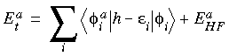
 . Specifically, the total energy Et may be written as:
Eq. 1
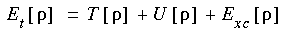 where T [] is the kinetic energy of a system of noninteracting particles of density , U [] is the classical electrostatic energy due to Coulombic interactions, and Exc [] includes all many-body contributions to the total energy, in particular the exchange and correlation energies. Eq. 1 is written to emphasize the explicit dependence of these quantities on (in subsequent equations, this dependence is not always indicated).
Wavefunction as antisymmetrized product of molecular orbitals
As in other molecular orbital methods (Roothaan 1951, Slater 1972, Dewar 1983), the wavefunction is taken to be an antisymmetrized product (Slater determinant) of one-particle functions, that is, molecular orbitals (MOs):
Eq. 2
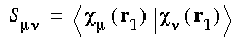
 The molecular orbitals also must be orthonormal:
Eq. 3
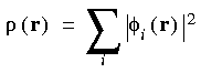
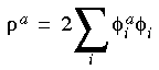
 The charge density
summed over all molecular
orbitals
The charge density
summed over all molecular
orbitals
In this case, the charge density is given by the simple sum:
Eq. 4
 Spin-restricted and -unrestricted
calculations
Spin-restricted and -unrestricted
calculations
where the sum goes over all occupied MOs
 i. The density obtained from this expression is also known as the charge density. The MOs may be occupied by spin-up (alpha) electrons or by spin-down (beta) electrons. Using the same i for both alpha and beta electrons is known as a spin-restricted calculation; using different i for alpha and beta electrons results in a spin-unrestricted or spin-polarized calculation. In the unrestricted case, it is possible to form two different charge densities: one for alpha MOs and one for beta MOs. Their sum gives the total charge density and their difference gives the spin density--the amount of excess alpha over beta spin. This is analogous to restricted and unrestricted Hartree-Fock calculations (Pople and Nesbet 1954).
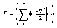
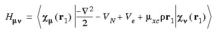
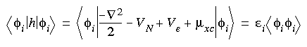
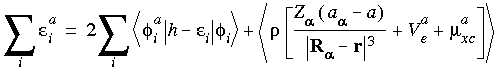
From the wavefunctions (Eq. 1) and the charge density (Eq. 4), the energy components can be written (in atomic units) as:
Eq. 5
Eq. 6
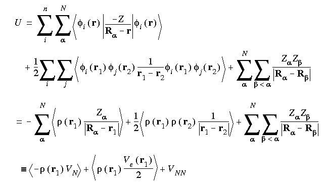 In Eq. 6, Z
 refers to the charge on nucleus of an N-atom system. The first term, VN , represents the electron-nucleus attraction. The second, Ve/2, represents the electron-electron repulsion. The final term, VNN , represents the nucleus-nucleus repulsion.
Approximating the exchange-correlation energy
The final term in Eq. 1, the exchange-correlation energy, requires some approximation for this method to be computationally tractable. A simple and surprisingly good approximation is the local density approximation, which is based on the known exchange-correlation energy of the uniform electron gas (Hedin and Lundqvist 1971, Ceperley and Alder 1980, Lundqvist and March 1983). Analytical representations have been made by several researchers (Hedin and Lundqvist 1971, Ceperley and Alder 1980, von Barth and Hedin 1972, Vosko et al. 1980, Perdew and Wang 1992). The local density approximation assumes that the charge density varies slowly on an atomic scale (i.e., each region of a molecule actually looks like a uniform electron gas). The total exchange-correlation energy can be obtained by integrating the uniform electron gas result:
Eq. 7
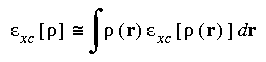 where Exc [] is the exchange-correlation energy per particle in a uniform electron gas and is the number of particles.
This implementation uses the form derived by Vosko et al. (1980), denoted the VWN functional, as the default. Other local spin-density functionals, developed by Von Barth and Hedin (BH), Janak, Morruzi, and Williams (JMW), and the latest Perdew and Wang work (PW), are also available when a nonstandard type of DMol calculation is chosen.
The next step in improving the local spin-density (LSD) model is to take into account the inhomogeneity of the electron gas which naturally occurs in any molecular system. This can be accomplished by a density gradient expansion, sometimes referred as the nonlocal spin-density approximation (NLSD). Over the past few years it has been well documented that the gradient corrected exchange-correlation energy Exc[
, d ()] is necessary for studying the thermochemistry of molecular processes (see recent reviews by Ziegler 1991, Labanowski and Andzelm 1991, Politzer and Seminario 1995).
In the present implementation, several commonly used NLSD functionals are available. The default is the Perdew and Wang (PW) generalized gradient approximation for the correlation functional and the Becke (B) gradient corrected exchange functional. This level of approximation for NLSD Hamiltonian is referred to as the BP functional. In addition, the gradient corrected correlation functional of Lee, Yang, and Parr (LYP) is available.
The total energy can now be written as:
Eq. 8

To determine the actual energy, variations in Et must be optimized with respect to variations in , subject to the orthonormality constraints in Eq. 2 (Kohn and Sham 1965):
where
 ij are Lagrangian multipliers. This process leads to a set of coupled equations first proposed by Kohn and Sham (1965):
Eq. 10
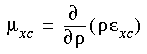
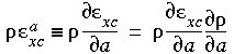
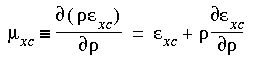
 The term µxc is the exchange-correlation potential, which results from differentiating Exc. For the local-spin density approximation, the potential µxc is:
Eq. 11
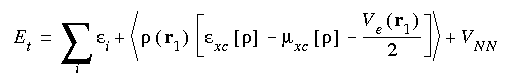
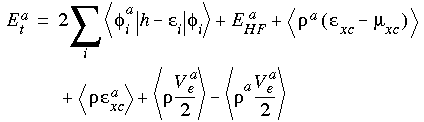
 Use of the eigenvalues of Eq. 10 leads to a reformulation of the energy expression:
Eq. 12
 Convenience of expanding
MOs in terms of AOs, or
basis functions
Convenience of expanding
MOs in terms of AOs, or
basis functions
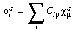
In practice, it is convenient to expand the MOs in terms of atomic orbitals (AOs):
Eq. 13
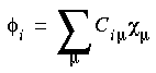 The atomic orbitals
  µ are called the atomic basis functions, and the Ciµ are the MO expansion coefficients. Because linear combinations of AOs are used, the Ciµ are also sometimes called the LCAO-MO coefficients. Several choices are possible for the basis set, including Gaussian (Andzelm et al. 1989), Slater (Versluis and Ziegler 1988), and numerical orbitals. In this implementation, numerical orbitals are used--these are discussed at some length under Numerical basis sets.
Unlike the MOs, the AOs are not orthonormal. This leads to a reformulation of the DFT Eq. 10 in the form:
Eq. 14
 where:
Eq. 15
 and:
and:
Eq. 16
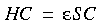
 SCF procedure
Because H depends upon C, Eq. 14 must be solved by an iterative technique. This can be done by the following procedure:
i.
 new - old < 10-6. For metallic systems, many more iterations are frequently required.
The basis functions
m are given numerically as values on an atomic-centered spherical-polar mesh, rather than as analytical functions (i.e., Gaussian orbitals). The angular portion of each function is the appropriate spherical harmonic Ylm( ,). The radial portion F(r) is obtained by solving the atomic DFT equations numerically. A reasonable level of accuracy is usually obtained by using a range of 300 radial points from the nucleus to an outer distance of 10 Bohrs (
 5.3 Å). Radial functions are stored as a set of cubic spline coefficients for each of the 300 sections, so that F(r) is actually piecewise analytic. This is an important consideration for generating analytic energy gradients. In addition to the basis sets, the -
 2/ 2 terms required for evaluation of the kinetic energy are also stored as spline coefficients.
The use of the exact DFT spherical atomic orbitals has several advantages. For one, the molecule can be dissociated exactly to its constituent atoms (within the DFT context). Because of the quality of these orbitals, basis set superposition effects (Delley 1990) are minimized, and an excellent description of even weak bonds is possible.
 4p excited state. Basis set quality has been analyzed in detail by Delley (1990).
Frozen core functions reduce computational cost
In all cases, the frozen-core approximation may be used. Core functions are simply frozen at the values for the free atoms, and valence orbitals are orthogonalized to them. Use of frozen cores reduces the computational effort by reducing the size of the secular equation (Eq. 10) without much loss of accuracy.
Numerical integration
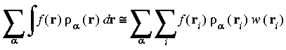
Evaluation of the integrals in Eqs. 15 and 16 must be accomplished by a 3D numerical integration procedure, due to the nature of the basis functions. The matrix elements need to be approximated by the finite sums:
Eq. 17
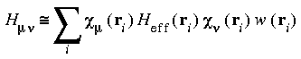
Eq. 18
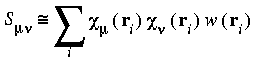 The sums run over several numerical integration points ri. The term Heff (ri) represents the value of the integrand of Eq. 15 at point ri and w(ri) represents a weight associated with each mesh point. Increasing the number of mesh points improves the numerical precision of the integral but also results in additional computational cost.
Atomic and molecular integration grids
Careful selection of a set of integration points is important for the quality of the calculation (Delley 1990, Ellis and Painter 1968, Boerrigter et al. 1988). In general, the grid used to generate the atomic basis set is not suitable for molecular calculations. The grid used for atomic basis sets can take advantage of spherical symmetry, which greatly simplifies matters. For molecules, it is necessary to be able to treat the rapid oscillations of the molecular orbitals near the nuclei and to avoid integration of the nuclei themselves because of the nuclear cusps (Delley 1990).
The integration points are generated in a spherical pattern around each atomic center. Radial points are typically taken from the nucleus to an outer distance of 10 Bohrs (
5.3 Å). The number of radial points within this distance is designed to scale with increasing atomic number. For example, Fe requires more points than C. The typical number of radial points NR for a nucleus of charge Z is:
Eq. 19
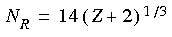 This number may, of course, be manually adjusted to accommodate the required precision or allowed cost of a calculation. The spacing between points is logarithmic--points are spaced more closely near the nucleus where oscillations in the wavefunction are more rapid.
Angular integration points N
are generated at each of the NR radial points, creating a series of shells around each nucleus. Angular points are selected by schemes designed to yield points ri and weights w(ri), which could yield exact angular integration for a spherical harmonic with a given value of l. Such quadrature schemes (Stroud 1971, Lebedev 1975 and 1977, Konyaev 1979) are available for functions up to l = 41. Alternatively, a product-Gauss rule in cos and may be used for arbitrary values of l (Stroud 1971). The product-Gauss methods use (l + 1) points on each shell, while the quadrature methods use more points:
| l |
N
|
|---|---|
| 5 | 14 |
| 7 | 26 |
| 11 | 50 |
| 17 | 110 |
| 23 | 194 |
| 29 | 302 |
| 35 | 434 |
| 41 | 590 |
Assuring consistent precision during integration
In practice, the quadrature method is used to generate the integration grid, and the product method is used as a check of numerical precision. On each radial shell, the sum of the atomic densities and the atomic electrostatic potentials is computed using both angular schemes. If the difference between the results of the two schemes is too large, then the next highest l value is used to generate a set of new points. This assures a consistent level of numerical precision throughout the integration grid. Typically, angular sampling increases when the difference between the two schemes is greater than 10-4. This yields
 1000 points per atom and offers a good compromise between computational cost and numerical precision.
Partition functions are used to increase the convergence of the numerical integration and to avoid integrating over nuclear cusps (Delley 1990, Hirshfeld 1977, Becke 1988). A partition function
a is defined as:
Eq. 20
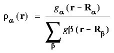 where is an atom index and g(r - R) is a function that typically is large for small r - R and small for large r - R (i.e., larger near the nucleus). Integrals are rewritten using partition functions as:
Eq. 21
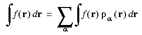 which is further reduced to a sum over 3D integration points:
Eq. 22
 Preferred partition function
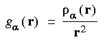
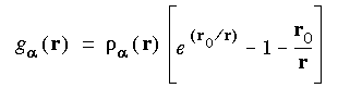
In practice, the partition functions are combined with the integration weights w(ri) to simplify the computation. The preferred choice for a partition function is:
Eq. 23
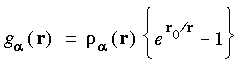 where r = |ri - R|, r0 = 0.5, and a is the atomic charge density for atom . Other options for partition functions include:
Eq. 24
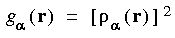
Eq. 25
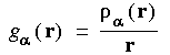
Eq. 26
Eq. 27
Evaluation of the effective potential
Evaluation of the exchange-correlation energy xc and potential µxc is accomplished with Eqs. 52, 55, and 57. This requires numerical evaluation of the charge density (r) at many points in space (i.e., xc and µxc are tabulated numerically). This restriction actually applies to most density function methods, even if analytical basis functions are used (Andzelm et al. 1989, Versluis and Ziegler 1988). The use of numerical basis functions facilitates this process, since all required quantities are already available on a grid of adequate numerical precision. An alternative approach (Baerends et al. 1973) is to fit the charge density to an analytic multipolar expansion via a least-squares fitting procedure. This simplifies the evaluation of xc and µxc, but still requires the use of a numerical grid for the least-squares fitting.
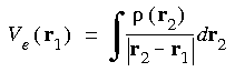
Evaluating the Coulombic potential numerically
The Coulombic potential is evaluated by solving the Poisson equation for the charge density:
Eq. 28
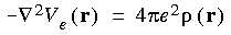 rather than by explicitly evaluating the Coulombic term as:
Eq. 29
 In the this approach, the Poisson equation is solved in a completely numerical (non-basis set) approach (Delley 1990). This provides greater numerical precision, since the evaluation of Ve is essentially exact once the form of (r) has been specified. Such a method requires specification of an analytic form of (r), as discussed above. However, rather than use a least-squares fitting procedure, a projection scheme is used. The charge density is first partitioned into atomic densities and then decomposed into multipolar components. Appropriate partition functions can ensure that such an expansion is rapidly convergent.
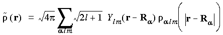
The density obtained in this way is called the model density. The term
alm r - R gives the model density for the multipolar component lm on atom for a shell at r - R distance from the nucleus:
Eq. 30
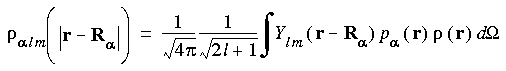 Note that the partition function p used for decomposition of the density is in general not the same as that used to improve the numerical integration in Eq. 22. The total model density is obtained from the summation over all alm:
Eq. 31
 Effect of angular truncation
on precision of model
charge density
Effect of angular truncation
on precision of model
charge density
The total model charge density is, in general, not equal to the orbital density
because of angular truncations. However, the flexibility of this model charge density is superior to that obtained with fitting procedures. The degree of angular truncation can be specified as an input parameter. Typically, a value of l one greater than that in the atomic basis provides sufficient precision; for example, the use of l = 3 truncation when p functions are present in the basis or l = 2 truncation if only p functions are used.
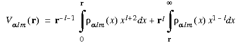
The Coulombic potential for each component is calculated using the Green function of the Laplacian (Delley 1990):
Eq. 32
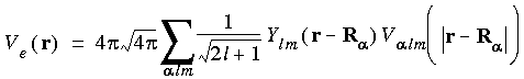
 The total potential
and the total potential is given by:
Eq. 33
Computational self-consistent field procedure
Interpolating the numerical
atomic bases onto the
molecular grid
Before the self-consistent field (SCF) procedure can be used, a step is required that is analogous to the evaluation of integrals over atomic orbitals, such as in Hartree-Fock methods. This is the interpolation of the numerical atomic basis set onto the molecular grid. Neglecting symmetry and any frozen-core approximations, this step requires a computational effort on the order of N X P for N atomic orbitals and P integration points. The basis set is controlled by the user, the number of points typically being on the order of 1000 points per atom. The overlap matrix (Eq. 16) and the constant portion of the effective Hamiltonian (Eq. 15) (kinetic and nuclear attraction terms) are constructed at this time, and each requires N X (N + 1) X P operations. The interpolated values can be stored externally and read as they are required. Alternatively, these data can be generated as needed, obviating the need for storage--this is termed a direct SCF procedure, by analogy with the direct Hartree-Fock method (Almlöf et al. 1982).
Constructing the initial molecular electron density
In practice, it is more convenient to skip Steps 1 and 2 (choosing an initial Ciµ and constructing an initial set of i, (see Choose an initial set of Cim.)) and to begin instead with an initial constructed from the superposition of atomic densities (quantities that are readily constructed from the numerical atomic basis set). In the SCF procedure, reconstruction of the new density requires a computational effort on the order of N X No X P, where No is the number of occupied orbitals.
Additional computational costs
Once
(r) is known, evaluation of the exchange-correlation potential µxc requires only P operations. Construction of the Coulombic potential requires only P X M effort, where M is the number of multipolar functions. M is typically on the order of 9 functions atom-1 (l = 2) or 16 functions atom-1 (l = 3). Neither of these steps is especially time consuming.
Reducing the computational cost
For large systems, the computational cost does not necessarily grow as rapidly as implied by the above comments. Since the atomic basis functions have a finite extent (
10 Bohrs), only a limited number of points contribute to each matrix element and P eventually converges to a constant. In addition, construction of the density and the secular matrix can be accomplished using sparse matrix multiplier routines, further reducing the computational cost.
Construction of a new density follows solution of the secular equation. Damping is usually required to ensure smooth convergence. In the current method, simple damping is possible:
Eq. 34
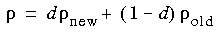 where d is the damping factor, old is the density that was used to construct the secular matrix, new is the density constructed from the new MO coefficients without damping, and is the density that is actually used in the next iteration. An interpolation/extrapolation scheme is available. This technique constructs an effective vector from old to new for the current iteration and for the previous iteration. The effective vectors are generally skew vectors. The point of closest approach between old and new is used to extrapolate the actual density for the next iteration. The Pulay DIIS method (Pulay 1982) has been implemented.
The direct inversion of the iterative subspace (or DIIS) method developed by Pulay (Pulay, 1982) has been implemented in DMol as a mechanism to speed up SCF convergence. The method rests on the suitable definition of an error vector that is zero when convergence is achieved and on performing a linear combination of a set of error vectors sampled along iterations that produces a new error vector with minimal norm. (This algorithm was present in previous versions of DMol, yet restricted to interpolation of at most two error vectors.) The DIIS method is much more powerful if one allows for a slightly larger dimension of iterative subspace. The default dimension currently adopted in DMol is 4. An upper limit of 10 was imposed in the current DIIS scheme, which is motivated by the fact that linear dependencies between error vectors and therefore the amount of redundant information increases with the size of the vector space.
Eq. 35
 The final model density is a linear combination of the densities at each SCF iteration i:
Eq. 36
 with the constraint that
  . The Ci coefficients are calculated by minimizing the norm:
Eq. 37
 where
where  .,l,m and numerical integration over all the molecular grid points.
The equations of density functional theory include an electrostatic potential arising from the negatively charged electron density. For more efficient calculations, the potential is found by solving the Poisson equation rather than by the equivalent approach of four-center direct integrals. Using the Poisson equation requires an auxiliary density representation ~, which is a function rather than the sum of squares of a function. ~ differs from (Eq. 4):
Eq. 38
 Effect of auxiliary density
approximation on accuracy
of calculated total
energy
Effect of auxiliary density
approximation on accuracy
of calculated total
energy
To minimize the impact of this difference a total-energy formula is used that is second-order in
 (Delley et al. 1983, Delley 1990, Delley 1991). The default starting density in DMol is the sum of the spherical atom densities. The total energy calculated in the first SCF cycle is thus the so-called Harris approximation (Harris 1985). The atomic dissociation energy in the first cycle is usually overestimated, since the electrostatic error term for the total energy:
Eq. 39
 is negative definite. The less important second-order term for local density functionals is positive definite, which leads to a slight overestimation of the total energy during the SCF iterations., is now:
Eq. 40
where  is the density for spin alpha and beta, respectively; ni
 are the occupations of orbitals with the orbital and spin labels i, ; i is the corresponding eigenvalue, which has been calculated using the static V~e and exchange-correlation potential µ~xc, arising from the spin densities ~. Exc is the exchange-correlation functional (local or nonlocal).
Energy gradients
Predicting chemical structure
The ability to evaluate the derivative of the total energy with respect to geometric changes is critical for the study of chemical systems. Without the first derivatives, a laborious point-by-point procedure is required, which is taxing to both computer and human resources. The availability of analytic energy derivatives for Hartree-Fock (Pulay 1969), CI (Brooks et al. 1980), and MBPT (Pople et al. 1979) theories (to name just a few) has made these remarkably successful methods for predicting chemical structures.
The derivative of the total energy in Eq. 12 with respect to a nuclear perturbation in direction a (x, y, or z) of atom may be written as:
Eq. 41
where the derivative density is defined as:
Eq. 42
 with:
with:
Eq. 43
 Derivative of the basis
function
Derivative of the basis
function
The derivative of the basis function
m with respect to the perturbation a can be computed analytically because of the representation of the numerical basis sets. The angular portion of m is a spherical harmonic function, which is analytic and easily differentiated. The radial portion is represented by several cubic splines, each of which is also differentiable.
The derivatives of the eigenvalues can be obtained from Eq. 10. Multiplying by i and integrating gives an expression for i:
Eq. 44
 Differentiating and rearranging yields:
Eq. 45
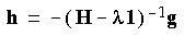
 The terms in Eqs. 45 and 49 involving Z represent the Hellmann-Feynman force (Hellmann 1939, Feynman 1939), which gives the derivative in the absence of any orbital relaxation.
Substituting Eq. 45 into Eq. 41 yields:
Eq. 46
 Where Eat is the Hellmann-Feynman term. Now (Andzelm et al. 1989):
Eq. 47
 and recalling the definition in Eq. 11, we can also write:
Eq. 48
 The final equation for the
derivative of the energy
The final equation for the
derivative of the energy
Therefore, the terms in Eq. 46 involving xc cancel. In addition, if Eq. 29 is used to construct the charge density, then the last two terms in Eq. 46 also cancel, leaving:
Eq. 49
 which is formally the same as the equation derived by other researchers (Andzelm et al. 1989, Versluis and Ziegler 1988). In practice, however, it is necessary to compute both Va/2 and aV/2, because the model density from Eq. 31 is not exactly equal to the numerical charge density computed from Eq. 4.
The time required to evaluate all 3N first derivatives for an N-atom system is typically the same as the time required for 3-4 SCF iterations. If convergence is achieved in, say, 10-12 iterations, then 25-30% additional time is required to evaluate the derivatives. Others have obtained similar results (Versluis and Ziegler 1988).
Because of numerical precision, two potential problems have been observed in evaluating gradients. First, the energy minimum does not correspond exactly to the point with zero derivative (Versluis and Ziegler 1988). The gradients are typically about 10-4 at the energy minimum. A second important point is that the sum of the gradients is not always zero, as it must be for translational invariance. The sum can be as high as 10-3 if the calculation is very poor. Increasing the quality of the integration mesh and the number of multipolar functions in the model density can reduce this to about 3.0 X 10⁻⁵. This magnitude of error seems to be permissible for geometry optimizations: the error introduced in the geometry is typically on the order of 0.001 Å. Only for very flat potential energy surfaces should this be a problem.
Currently, the geometry is optimized using both Cartesian and internal coordinates (see Geometry optimization -- The OPTIMIZE suite of algorithms). When the geometry is optimized under conditions of symmetry, only forces that maintain molecular symmetry are evaluated, resulting in considerable time savings. Even in the absence of symmetry, certain forces can be omitted from the calculation, resulting in faster calculations. For example, for a substrate adsorbed on a metal cluster, it is possible to compute gradients for the substrate only and perform no optimization on the metal.
Electron gas model
The equations actually
used in DMol
The parameterized equations for the electron gas exchange-correlation energy as used in DMol are presented explicitly in this section. An excellent review of the electron gas model can be found in Appendix E of Parr and Yang (1989). As mentioned earlier, the implementation in DMol is based on the work of von Barth and Hedin (1972).
Eq. 50
 The exchange energy
Then the exchange energy is given by:
Eq. 51
 where:
Eq. 52
 Spin-restricted computations
The correlation contribution depends upon whether this is a spin-restricted or unrestricted computation. For a restricted computation, the correlation contribution is given by:
Eq. 53
 where:
 Spin-unrestricted computations
For a spin-unrestricted computation, the expression is:
Eq. 55
 where:
Eq. 56
 and:
and:
Eq. 57
DMol supports most of the chemically important symmetry point groups. If, however, a system is selected with a point group that is not supported, DMol automatically switches to the highest-order subgroup. The Cn, Cnh, and S2n groups are not supported yet, because the complex character tables are not available in DMol. The rotational groups C
Point-group symmetry v and Dh are also not supported yet, but such systems can be computed in C6v and D6h, respectively, without major loss in efficiency. The supported groups are:
	C1	Cs	Ci
	C2	C2v     C2h      D2      D2h     D2d
		C3v		D3	D3h	D3d
		C4v		D4	D4h	D4d
		C5v		D5	D5h	D6d
		C6v		D6	D6h	D5d
		Td	O	Oh	I	Ih
After this introductory section, the theory behind the principal algorithms in OPTIMIZE is presented, starting under Theory and implementation. (This section can be skipped by those whose sole interest is how to use the program.) Methodology--Insight, includes a discussion of input parameters, options, and how to use OPTIMIZE within the Insight interface. Lessons demonstrating how to use the Optimize/Opt_Parameters command are described in Tutorial--The Insight Environment.
OPTIMIZE is a general geometry-optimization package for locating both minima and transition states on a potential energy surface. It can optimize in Cartesian coordinates or in a nonredundant set of internal coordinates that are generated automatically from input Cartesian coordinates. It also handles fixed constraints on distances, bond angles, and dihedral angles in Cartesian or (where appropriate) internal coordinates.

|
OPTIMIZE is designed to operate with minimal user input. All you need to provide is the initial geometry in Cartesian coordinates (obtained from the Insight or Discover programs or from an appropriate database), the type of stationary point sought (minimum or transition state), and details of any imposed constraints. All decisions as to the optimization strategy--how to handle the constraints, whether to use internal coordinates, which optimization algorithm to use--are made by OPTIMIZE.
The heart of the program (for both minimization and transition-state searches) is the EF (eigenvector-following) algorithm (Baker 1986). The Hessian mode-following option incorporated into this algorithm is capable of locating transition states by walking uphill from the associated minima. By following the lowest Hessian mode, the EF algorithm can locate transition states, starting from any reasonable input geometry and Hessian.
An additional option available for minimization is GDIIS, which is based on the well known DIIS technique for accelerating SCF convergence (Pulay 1982).
The strategy adopted for constrained optimization depends on the starting geometry and the nature of the constraints. Constraints can be handled easily in internal coordinates, provided that (1) the constrained parameter (distance, angle, or dihedral) is a natural part of the coordinate set and (2) the constraint is rigorously satisfied in the starting structure. If both (1) and (2) hold for all desired constraints, then OPTIMIZE carries out the optimization in internal coordinates. Otherwise, the constrained optimization is performed in Cartesian coordinates.
Traditional wisdom has it that optimization in Cartesian coordinates is inefficient relative to internal coordinates; however, recent work (Baker and Hehre 1991) has clearly demonstrated that, if a reasonable estimate of the Hessian matrix is available (e.g., from a molecular mechanics forcefield) at the starting geometry, then optimization directly in Cartesian coordinates is as efficient as an internal coordinate optimization. In particular, constrained optimization can be handled in Cartesian coordinates as efficiently as with a Z-matrix, with the additional advantages that any distance, angle, or dihedral constraint between any atoms in the molecule can be dealt with (i.e., there is no formal connectivity requirement), and the desired constraint does not have to be satisfied in the starting structure.
OPTIMIZE incorporates a very accurate and efficient Lagrange multiplier algorithm for handling constraints in Cartesian coordinates, with a more robust (but less efficient) penalty function algorithm as a backup. Both algorithms are suitably modified versions of the basic EF algorithm (Baker 1992). The Lagrange multiplier code can locate constrained transition states, as well as minima.
Theory and implementation
The EF algorithm and mode following
Shifting the Newton-
Raphson step to favor
optimization along an
eigenmode
Mode following is a powerful technique for geometry optimization. It involves modifying the standard Newton-Raphson step:
Eq. 58
 by introducing a shift parameter
  so that (Cerjan and Miller 1981):
Eq. 59
 In terms of a diagonal Hessian representation, this can be written:
Eq. 60
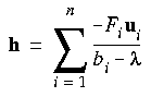 where the ui and bi are the eigenvectors and eigenvalues of the Hessian matrix H, and
  = uti g is the component of g along the local eigenmode ui. Scaling the Newton-Raphson step in this way has the effect of directing the step to lie primarily (but not exclusively) along one of the local eigenmodes, depending on the value chosen for .
Various recipes for choosing a suitable shift parameter exist: the EF algorithm utilizes a rational function approximation to the energy, yielding an eigenvalue equation of the form (Banerjee et al. 1985):
Eq. 61
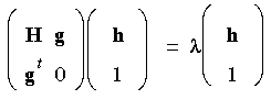 from which a suitable can be obtained. This RFO matrix equation has the following important properties:
i} bracket the n eigenvalues {bi} of the Hessian matrix i bi i+1.
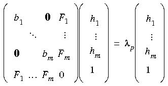
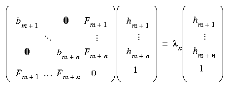
Property 3--the separability of the positive and negative Hessian eigenvalues--allows two shift parameters
p and n to be used, one for modes along which the energy is to be maximized and the other for which it is minimized. Specifically, for a transition state (a saddlepoint of order 1) in terms of the Hessian eigenmodes, we have the two matrix equations:
Eq. 62
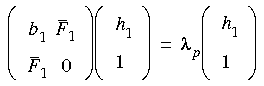
Eq. 63
 where it is assumed that maximization is along the lowest Hessian mode bi. Note that p is the highest eigenvalue of Eq. 62--it is always positive and approaches zero at convergence--while n is the lowest eigenvalue of Eq. 63--it is always negative and again approaches zero at convergence.
Choosing these values of gives a step that attempts to maximize along the lowest Hessian mode and minimize along all the others. It always does this regardless of the eigenvalue signature (unlike the standard Newton-Raphson step). The two shift parameters are then used in Eq. 61 to give a final step:
Eq. 64
 This step may be further scaled down if it is considered too long. For minimization, only one shift parameter n would be used and this would act on all modes. It is often possible to locate different transition states from the same starting structure by maximizing along a mode other than the lowest (hence "mode following").
Constrained optimization
Lagrange multipliers as
constraints
The essential problem in constrained optimization is to minimize a function of, say, n variables F(x) subject to a series of m constraints of the form Ci (x) = 0, (i = 1 ... m). This can be handled by introducing the Lagrangian function (Fletcher 1981):
Eq. 65
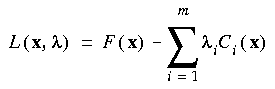 which replaces the function F(x) in the unconstrained case. Here, the i are the so-called Lagrange multipliers, one for each constraint Ci(x). Taking the derivative of Eq. 65 with respect to x and gives:
Eq. 66
 and:
and:
Eq. 67
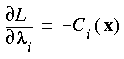 At a stationary point of the Lagrangian function, we have L = 0, that is, all
  L/xj = 0 and all L/i = 0. This latter condition means that all Ci (x) = 0, and so all constraints are satisfied. Hence, finding a set of values (x, ) for which L = 0 gives a possible solution to the constrained optimization problem in precisely the same thing as finding an x for which g = F = 0 gives a solution to the corresponding unconstrained problem.
We can implement mode following in constrained optimization by simply adopting Eq. 61, but with H replaced by 2L and g replaced by L. However, it is important to realize that each constraint introduces an additional mode to the Lagrangian Hessian (2L), which has negative curvature (a negative Hessian eigenvalue). Thus, when considering minimization with m constraints, you should look for a stationary point of the Lagrangian function whose Hessian has m negative eigenvalues, that is, for a saddle point of order m.
Insofar as mode following is concerned then, assuming a diagonal Lagrangian Hessian representation, Eqs. 62 and 63 for an unconstrained system should be replaced by the following for a constrained system:
Eq. 68
Eq. 69
 where now the bi are the eigenvalues of 2L with corresponding eigenvectors ui and
  = uti L. Constrained transition-state searches can be carried out by selecting one extra mode to be maximized in addition to the m constraint modes, that is, by searching for a saddlepoint of the Lagrangian function of order m + 1.
GDIIS
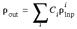
In the GDIIS method, geometries (xi) generated in previous optimization steps are linearly combined to find the "best" geometry on the current cycle (Császár and Pulay 1984):
Eq. 70
 Finding appropriate coefficients
for use in GDIIS
method
Finding appropriate coefficients
for use in GDIIS
method
The problem here, of course, is to find appropriate values for the coefficients Ci.
Eq. 71
 and:
and:
Eq. 72
 are satisfied, then the relation:
Eq. 73
 also holds.
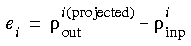
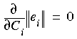
The true error vectors ei are, of course, unknown. However, they can be approximated by:
Eq. 74
 where gi is the gradient vector corresponding to the geometry xi. Minimization of the norm of the residuum vector (Eq. 71), together with the constraint equation (Eq. 72), leads to a system of m + 1 linear equations:
Eq. 75
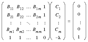 where Bij =
  ei ej
ei ej is the scalar product of the error vectors ei and ej, and is a Lagrange multiplier.
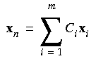
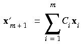
The coefficients Ci determined from Eq. 75 are used to calculate an intermediate interpolated geometry:
Eq. 76
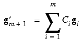
 and its corresponding interpolated gradient:
Eq. 77
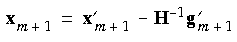
 Relaxing the intermediate
geometry
Relaxing the intermediate
geometry
A new, independent geometry is generated by relaxing the interpolated geometry according to:
Eq. 78
 Modifications of the original
GDIIS algorithm
Modifications of the original
GDIIS algorithm
In the original GDIIS algorithm, the Hessian matrix is static, that is, the original starting Hessian remains unchanged during the entire optimization. However, updating the Hessian at each cycle generally results in more rapid convergence, and this is the default in OPTIMIZE. Other modifications to the original method include limiting the number of previous geometries used in Eq. 70 by neglecting earlier geometries and eliminating any geometries more than a certain distance (default = 0.3 au) from the current geometry.
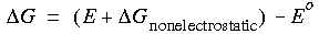
The DMol module in release 4.0.0 of the Insight program includes some COSMO controls, which allow for the treatment of solvation effects.
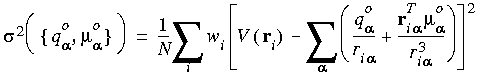
COSMO--solvation effects that represents the solvent: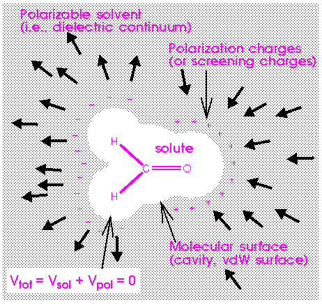 ) = ( - 1) / ( + 1/2), to obtain a rather good approximation for the screening charges in a dielectric medium.
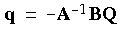
  2 they may reach 10% of the total screening effects. However, for weak dielectrics, screening effects are small, and the absolute error therefore amounts to less than a kilocalorie per mole. + Z for the total solute charges such as electron density and nuclear charges Z, then the vector of potentials Vtot on the surface is Vtot = BQ + Aq = Vsol + Vpol, where BQ is the potential arising from the solute charges Q, and Aq is the potential arising from surface charges q. B and A are Coulomb matrices. For a conductor, the relation Vtot = 0 must hold, which defines the screening charges as:
Eq. 79
 For further details of the COSMO theory see Klamt and Schüürmann (1993). COSMO provides the electrostatic contribution to the free energy of solvation. In addition, there are nonelectrostatic contributions to the total free energy of solvation, which describe the dispersion interactions and cavity formation effects.
DMol/COSMO
The COSMO electrostatic energy is analogous in form to the DMol electrostatic energy, with the Coulombic operator replaced by the dielectric operator D = BA-1 B. From Eq. 40 we can write:
Eq. 80
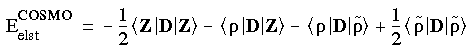 where
where  represents the auxiliary density, which is introduced to solve the Poisson equation for the electrostatic potential of the solute. This total energy is minimized, resulting in the Kohn-Sham equations for the molecular orbitals. The Kohn-Sham Hamiltonian now includes an electrostatic COSMO potential:
Eq. 81
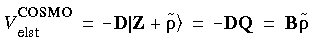 This potential is present in every SCF cycle. This direct incorporation of the solvent effects within the SCF procedure is a major computational advantage of the COSMO scheme. Since the DMol/COSMO orbitals are obtained using the variational scheme, we can derive accurate analytic gradients with respect to the coordinates of the solute atoms. The complete theory is presented in Klamt and Schüürmann (1993) and Andzelm et al. (1995). The gradients include the forces between the solute charges Q and the screening charges q.
The DMol/COSMO method has been tested extensively (Klamt and Schüürmann 1993, Andzelm et al. 1995). The results depend mainly on the choice of the van der Waals radii used to evaluate the cavity surface. The other parameters defining the cavity surface (see below) are less important. Of course, solvation energies depend on the choice of DMol parameters, such as the type of DFT functional, the basis set, and integration grid. Results obtained so far (Andzelm et al. 1995) suggest that the DMol/COSMO model can predict solvation energies for neutral solutes with an accuracy of about 2 kcal mol-1.
Determination of the cavity surface (or solvent-accessible surface)
The surface is obtained as a superimposition of spheres centered at the atoms, discarding all parts lying on the interior part of the surface (Klamt and Schüürmann 1993). The spheres are represented by a discrete set of points, the so-called basic points. Eliminating the parts of the spheres that lie within the interior part of the molecule thus amounts to eliminating the basic grid points that lie in the interior of the molecule.
Determination of nonelectrostatic contributions to the free energy of solvation
The free energy of solvation is calculated as:
Eq. 82
 where Eo is the total DMol energy of the molecule in vacuo, E is the total DMol/COSMO energy of the molecule in solvent, and
  Gnonelectrostatic is the nonelectrostatic contribution due to dispersion and cavity formation effects. The nonelectrostatic contributions to the free energy of solvation are estimated from a linear interpolation of the free energies of hydration for linear-chain alkanes as a function of surface area:
Eq. 83
Gnonelectrostatic = A_Constant + B_Constant * surface_area
In the present implementation, the VWN potential, DNP basis set, and fine integration grid of DMol were used to calculate energies of methane and octane (C2h). The experimental values of the free energy of solvation are 1.9 and 2.9 kcal mol-1 for methane and octane, respectively (Ben-Naim and Marcus 1984). The default (see next section) set of COSMO parameters was chosen. The calculated surface areas were 38.4 and 104.1 Å2 for methane and octane, respectively. The following values of A_Constant and B_Constant were used:
Gnonelectrostatic by as much as 0.5 kcal mol-1.
Derivation
The electric field gradient is defined as the gradient of the electric field and is therefore the second derivative (or Hessian) of the electrostatic potential at a given position:
Eq. 84
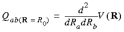 where R0 = position at which the derivative is evaluated, Q = electric field gradient, V = electrostatic potential, R = general position vector, and a, b = x, y, or z.
Eq. 85
 The trace of Q defined as above yields (Poisson equation):
Eq. 86
 with = the charge density.
Eq. 87
 In DMol, the tensor Q is computed through expanding the electrostatic potential into a Taylor series with respect to each of the nuclei (if symmetry is imposed, only the symmetry-unique nuclei are visited). The matrix Q then appears as the coefficient of the second-order term in the Taylor expansion:
Eq. 88
 Uses
Uses
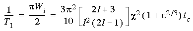
The energy of an electrostatic quadrupole moment embedded in an electrostatic potential is determined by the electric field gradient at the position of the quadrupole. This interaction contributes to the NMR line width (as further outlined below).
The electric field gradient at a quadrupolar nucleus (spin I > 1/2) within a molecule determines the NMR longitudinal relaxation rate 1/T1 or the line width W1/2 (this assumes that the quadrupolar relaxation mechanism dominates):
Eq. 89
|
Miyake et al. (1996) use a different formula, in which enters into the equation as (1 + 2)/3.
|
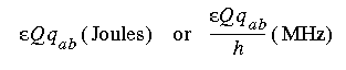
In Eq. 89, I = nuclear spin quantum number (e.g., I = 1 for 14N, I = 5/2 for 17O, I = 3/2 for 33S, I = 7/2 for 45Sc), = nuclear quadrupolar coupling constant and is = 2 Q qzz/h, where qzz = largest principal component of the EFG tensor q, (asymmetry parameter) = |qxx - qyy|/qzz, and the x, y, z axes are chosen such that || < 1. (Since enters into the relaxation time as 2, the sign of is not important and may be dropped (Bagno & Scorrano 1996).)
tc = rotational correlation time and can be estimated from the Debye-Stokes-Einstein formula as tc = Vm
 /(kT), where Vm = hydrodynamic volume (= 4 (
 /3) R3, where R = hydrodynamic radius) and = solution viscosity.
Eq. 90
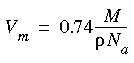 where M = molecular weight, = solute density, and Na = Avogadro's number.
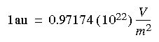
The EFG in atomic units can be converted to SI units with the conversion factor:
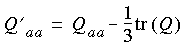
 Q is the maximum expectation value of the zz traceless tensor element:
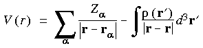
The ESP is generated in the space of a molecule and can be calculated from the positions of the atomic nuclei
and the electron density :
 Practical implementation of the fitting technique in DMol requires first, calculation of the ESP on a three-dimensional rectangular grid that covers the molecule. The extension of the grid ri is determined by the atomic radii as will be explained in detail below.
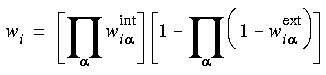
The values of the atomic multipoles are obtained by minimizing the following expression for the mean square deviation between the calculated ESP and the model potential due to the atomic multipoles:
 where wi are the point weights and
  ,
,  are the atom-centered charges and dipoles, respectively.
 The current release of DMol allows for fitting only charges centered on the nuclei. The total molecular charge is conserved, using the Lagrange multiplier technique.
The grid points in Eq. 92 are selected based on the following criteria:
Eq. 93
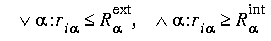 where
where  and
and  are the internal and external radii of the atomic shells and depend on the atom type.
Eq. 94
 where
where  and
and  are the partial weights calculated with respect to all ESP centers in the system:
Eq. 95

Eq. 96
 where R is the "diffusion" width of the layer border.
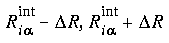 and from 1 to 0 across the external radii
  .
.
The measurement of optical absorption spectra yields information about the difference between energy levels and about the intensity of the transition between energy levels, which is related to the strength of the coupling with the external electric field inducing the transition.
Optical absorption spectra
If the initial state of lower energy is denoted as
 with energy Ei, and the final, excited state of higher energy is denoted as
  with energy Ef, an absorption band should be observed at an energy:
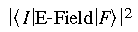 IE-FieldF describes the strength of the coupling between the two states I and F mediated by the electric field E-Field. E-Field is a three-dimensional vector with components Ex, Ey, Ez.IE-FieldF is different from zero, the transition between states I and F is called a dipole transition. Computation of the matrix element is equivalent to computing the transition moment between states I and F, which is given as IrF, where r is a general three-dimensional vector with components x, y, and z.X is given by X-erX where e is the unit of charge. If the matrix element is zero, transitions may still be observable as multipole (quadrupole, etc.) transitions.
I is a Slater determinant formed by the occupied Kohn-Sham orbitals.
IE-FieldF would otherwise vanish. Such a transition is called spin forbidden.The second assumption is quite drastic in that it assumes that the excited state can be described by the Kohn-Sham orbitals of the ground state. This ignores both relaxation effects and more fundamental problems describing excited states within density functional theory (Slater 1972, Hedin 1965, Hybertsen & Louie 1986). (Slater transition state theory (Slater 1972) can be performed for particular transitions; however, it does not allow for rapid evaluation of the optical absorption spectrum.)
Implementation
The algorithm for the computation of optical absorption spectra within DMol is:
Loop over all occupied orbitals |i>
     Loop over all unoccupied orbitals |a>
          Compute Energy difference dE = Ea - Ei
          Compute Matrix elements <i|x,y,z|a>
     End Loop
End Loop
where the occupied Kohn-Sham orbitals are i with orbital energies Ei, and the unoccupied Kohn-Sham orbitals are a with orbital energies Ea.This double loop is executed for both sets of orbitals for a calculation with unrestricted spin.
Transition moments and symmetry
The computation of transition moments can be made more efficient if the molecular system under consideration possesses symmetry. If it does, selection rules can be applied to avoid computation of matrix elements that are known to be zero on the basis of symmetry arguments alone. The transitions that are not allowed due to symmetry are called symmetry-forbidden. It is possible, of course, that a matrix element is symmetry-allowed but turns out to be zero nevertheless. This happens, for example, when the calculation utilizes only a subgroup of the actual point group of the molecular system.
ix,y,za to be different from zero, it has to be invariant to any symmetry operation that transforms the nuclear framework of the molecule into itself on the product i X (x,y,z) X a. Since it is known how the Kohn-Sham orbitals i,a and how the general three-dimensional position vector r = (x,y,z) transform when applying these operations, it is possible to tell whether the product is invariant. If the product is not invariant, the matrix element must be zero.+x,y+ and +z-, while all combinations +z+ and +x,y- are zero and need not be computed explicitly.
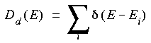 For analysis of metallic systems, some sort of artificial broadening is usually applied to the DOS plot. This results in a better match with experimental data obtained from methods like UPS and XPS. Two common ways of doing this are Gaussian and Lorentzian broadening. For Gaussian broadening every energy level is convoluted with a function like:
 For Lorentzian broadening we use the function:
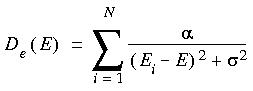 The sigma parameter indicates the width of the peaks. For sigma values approaching zero, we obtain the delta representation from Eq. 97. The value of sigma is typically varied so as to best represent the available experimental data.
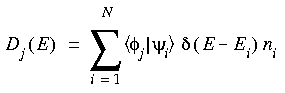
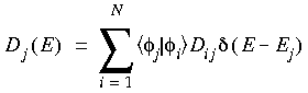
Partial density of states (PDOS), also called local density of states, can be used to study the contribution of a particular orbital or group of orbitals to the molecular orbital spectrum. These methods are based on different population analysis schemes such as the Mulliken and Loewdin methods.
Eq. 100
 This does give a reasonable indication of the contribution of that AO to the MO, but a major disadvantage is that the values are not normalized. Adding up the partial DOS for all orbitals in the system does not add up to the total number of electrons of the system, because of the non-orthogonality of the basis functions on different atoms.
Eq. 101
 where Dij is the AO density matrix. This definition allows the Mulliken density of states to become negative. The Loewdin analysis does not have this drawback, since, because of its definition, it always gives positive values:
Eq. 102
 where Sif = i | i and S1/2 is the square root of the overlap matrix S. However, we should stress that these different population analysis methods are all somewhat arbitrary, due to the partitioning of S, and care should be taken in attributing too much physical significance to them.
The concept of bond order and valence indices is well established in chemistry. It allows for interpretation and deeper understanding of the results of DMol calculations using ideas familiar to chemists.
Mulliken and Mayer bond orders is a molecular orbital and Ciµ are the SCF expansion coefficients then:
Eq. 103
 and matrix Pµ
 and a set of atomic orbitals completely specify the charge density (Eq. 42).
The trace of matrix P and the overlap S is equal to the total number of electrons in the molecule:
Eq. 104
 Summing (PS)µ contributions over all µ
  A, B , where A,B are centers, we can obtain PAB, which can be interpreted as the number of electrons associated with the bond A-B. This is the so-called Mulliken population analysis (Mulliken, 1955). The net charge associated with the atom is then given by:
Eq. 105
 where ZA is the charge on the atomic nucleus A.
 where P, P
 are the density matrices for spin and .

 where PS = P - P.
The Mayer bond orders and valence indices have several useful properties:
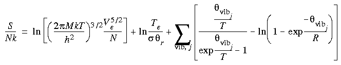
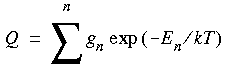 where the sum runs over all states n of total energy En and degeneracy gn, k is the Boltzmann constant (k = R/Na), and T is the absolute temperature.
All thermodynamic quantities can be derived from Q. For actual computations, several approximations have to be made:
The separation of electronic contributions is justified where the Born-Oppenheimer approximation is justified for calculating potential energy surfaces.
Eq. 110
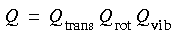 where Qtrans = translational contribution, Qrot = rotational contribution, and Qvib = vibrational contribution.
The translational partition function
The translational partition function is:
Eq. 111
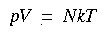
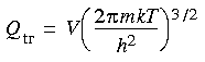 where V = volume (for an ideal gas, related to pressure according to V = RT/p), m = molecular mass, k = Boltzmann factor, T = absolute temperature, and h = Planck's constant.
The vibrational partition function is, within the harmonic oscillator approximation:
Eq. 112
 which is a product over all vibrations i with degeneracy di (di = 1 for non-degenerate vibrations) and frequency
  i (in wavenumber units); c is the velocity of light, which couples wavelength and frequency as c = .vib associated with a particular vibration j is defined as:
Eq. 113
 where k is the Boltzmann constant.
The computation of the rotational partition function under the assumption of a rigid nuclear framework (rigid rotor, ignoring couplings between rotational and vibrational motion) requires determination of the moments of inertia. The 3 X 3 moments of inertia tensor M is defined as:
Eq. 114
 where mk = mass of atom k; rk = position vector of atom k relative to the center of mass; and a,b = Cartesian components x,y,z.
Eq. 115
 According to equalities among the three moments of inertia IA, IB, and IC with respect to the principal axes, the molecule is classified as either:
 where B = h/(8 2 c IB), taking IA = 0, IB = IC.
For nonlinear molecules, we get:
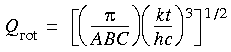 where A,B,C = h/(8 2 c I(A,B,C)).
This general expression covers the types of rotors described above.
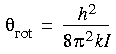
The characteristic rotational temperature
rot associated with a particular moment I is defined as:
 Approximate accounting
for nuclear spin: the symmetry
number
Approximate accounting
for nuclear spin: the symmetry
number
The coupling between nuclear spin and molecular rotation follows the same principle as the coupling between the electron spin and the electronic wavefunction. It is a quantum effect, but can be explained by a classical argument, resulting in the assignment of the so-called symmetry number.
Eq. 119
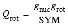 where SYM, the additional factor, is the symmetry number.
Given that electronically excited states are neglected, the ground state does contribute to the partition function if it is degenerate and if a special convention for the zero of the total energy is adopted.

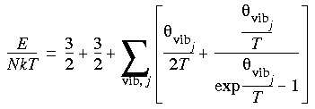
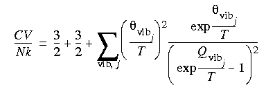
Thermodynamic quantities
Once the partition function Q is obtained, thermodynamic quantities can be derived. We have to emphasize again that these apply only to molecular gases (where intermolecular interactions are negligible) at temperatures that are neither too low (so that quantum effects are negligible) nor too high (so that the rigid rotor/harmonic oscillator approximation is applicable).

Eq. 120

Eq. 121

Eq. 122

Eq. 123
Eq. 124
 Nonlinear polyatomic
molecules
Nonlinear polyatomic
molecules
Eq. 125
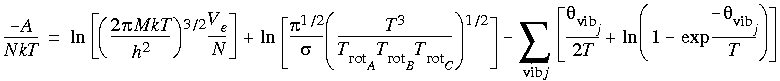
Eq. 126
Eq. 127
Eq. 128
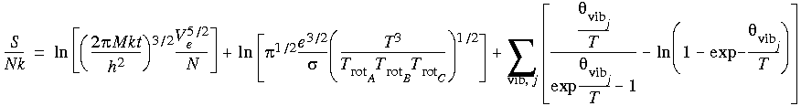
Eq. 129
 where e = Euler constant (ln e = 1), N = Avogadro's number, k = Boltzmann constant, and
  = characteristic rotational temperature (P = A,B,C).
Implementation
Thermodynamic quantities are calculated either as part of the quantum background job without additional user input (Turbomole, DMol) or as part of the analysis capabilities of the Insight Turbomole or DMol module, using the Analyze/Stat_Mech command.

