E
Commands--Standalone Mode

The following section contains a complete description of the commands used in the standalone version of DMol and illustrates how the command input file is set up and used. The commands are listed in alphabetical order.
Two input formats are possible in the standalone mode of DMol. The first type, where data goes to run_name.input, has a simplified format and allows almost the same flexibility as the other (.inmol) file. The second, which is written to run_name.inmol, requires fixed data format. This is the input format developed by the original authors.
You would probably find the .input format more useful. DMol searches first for .input and reads an .inmol file only if .input is absent. You can construct either of these files with a text editor, but the dialog and dmol_master interfaces (see Methodology--Standalone Mode) assist in writing .input files. In addition, dmol_master allows you to both set up and run DMol jobs. The dialog and dmol_master interfaces have some limitations with respect to some nonstandard options, as specified in the help for the dialog interface.
The rest of this section contains detailed descriptions of each of the commands available in the standalone version. For each command, documentation is divided into subsections.
Conventions used in documenting the commands are described below, along with a short description of the intent of each subsection.
Syntax
The Syntax subsection begins with the command syntax presented in as generic a form as possible. Several type style conventions are used to distinguish different kinds of words. For example:
command_keyword [value_keyword, ..., value_number, ...]
Words (or letters) in bold and not italicized indicate the names of keywords that must be typed exactly as shown. However, they are case-insensitive and may be typed in lower-, upper-, or mixed case.
A hash mark (#) at the beginning of a line indicates a comment line. It can also be used to temporarily comment-out a command.
Words in bold italics indicate options that must be replaced with appropriate text, as indicated in the table of allowed values that follows the syntax line for each command.
The values appropriate to each keyword are also listed and may be (as appropriate) numbers or enumerated constants:
Optional item(s) are enclosed in square brackets ([ ]), and, if there is more than one, the items are separated by commas. Ellipses (...) indicate that a kind of item may be repeated. The brackets, commas, and ellipses themselves are used for documentation only and should not be included in the real command.
Keywords are documented in alphabetical order. For a functional classification, please see Command Summary--Standalone Mode.
Basis allows you to specify the atomic basis set. This is the number and type of atomic orbitals used in the expansion of the molecular orbitals.
Basis value_keyword
[value_number ...
blank line]
The DND basis is comparable to Gaussian 6-31G* basis sets, and DNP basis sets are comparable to 6-31G** sets.
Minimal basis sets are generally inadequate for anything but qualitative results, while DNP sets are the most reliable. The .basis file contains at least a DNP basis for each atom up to Xe. You can also do calculations for heavier atoms (up to U). The fzminpol.dat file allows flexibility in choosing frozen orbitals, minimal basis sets, and polarization functions for these atoms (Atomic information supplied with DMol). For some atoms, triple-zeta basis sets and/or diffuse orbitals are provided. See Basis set summary for a complete list of the basis functions provided for each atom. Normally in a calculation, all of these orbitals are read in from the .basis file, which can be created by DAtom or directly by DMol. The min, dn, dnd, and dnp options operate by instructing the program to ignore the extraneous functions. This is reflected in the output file when certain orbitals may be designated as eliminated from the basis set.
When user is specified, you can specify exactly which orbitals in the .basis file are to be retained, dropped, or treated as frozen core. (The user option can be used to select more versatile combinations of frozen core orbitals than are possible with keyword Frozen.) Starting on the line immediately after the keyword Basis line, enter the data for each unique atom type (i.e., for each different atomic number) in the same order that the atoms appear in the Geometry specification. The data have the format:
nfrz nnls(i), i=1,nfrz
nfrz is the number of atomic basis functions on the atom, and nnls(i) tells DMol how to treat the i-th basis function of that atom.
- nnls(i) = 0 means include basis function #i in the calculation.
- nnls(i) = 1 means treat basis function #i as a frozen core.
- nnls(i) = 2 means delete this basis function entirely.
Repeat nfrz and nnls for each atom type, and terminate the list with a blank line.
As an example of user-specified basis sets, in Utilities, note that the .basis file contains the following functions for hydrogen:
1s 1s' 2p 2p' 2s
and for carbon:
1s 2s 2p 2s' 2p' 3d 2p'' 1s' 3d' 2p'''
Consider a calculation on CH2, with the H atoms appearing first in the Geometry specification. To obtain the same result as the DN specification using the user option, use the input:
Basis		user
 5 0 0 2 2 2
10 0 0 0 0 0 2 2 2 2 2
<BLANK LINE>
This input tells the program to delete all basis sets from hydrogen except 1s and 1s' and to delete everything from carbon except the 1s, 2s, 2p, 2s', and 2p'.
As a second example, consider the input:
Basis		user
 5 0 0 0 2 2
10 1 0 0 0 0 0 2 2 2 2
<BLANK LINE>
This specifies a DNP basis, since functions up to 2p are retained on H and those up to 3d are retained on C. The input in this example freezes the 1s core on C.
The Bond_Order keyword allows for calculation of the Mulliken and Mayer bond orders and valence indices.
Bond_Order value
This option allows for useful analysis of bond and valence indices, which can be correlated with classical chemistry concepts of bond and reactivity.
Bond orders can be calculated only for systems with C1 symmetry
The value of Calculate tells DMol which type of calculation you want to perform.
Calculate value_keyword
The Calculate keyword selects the type of calculation to perform. You provide one of the options from the above, for example:
Calculate frequency
The Charge keyword specifies the total molecular charge.
Charge value
When Charge and Occupation default are specified, DMol automatically chooses appropriate occupations for a neutral or ionic species.
If a user-specified occupation is used (Occupation valence or Occupation total), then Charge is automatically overridden: the total number of electrons specified by the user input is counted and used to determine the charge.
Constraint
constraint specifications ...
Endcon
The Constraint keyword is used to specify the distance, angle, and dihedral angle constraints that are to be enforced during a geometry optimization. The constraint specifications are input on separate lines of the input file (immediately following the line containing the Constraint keyword) and are specified as:
atom_i atom_j                    distance
atom_i atom_j atom_k             angle
atom_i atom_j atom_k atom_l      dihedral
Endcon
Where the atoms are indexed by integers in the order in which they appear in the molecular geometry, distances are expressed in angstroms, and bond angles and dihedral angles are expressed in degrees. The constraint specifications must be terminated with a separate line containing only the string Endcon immediately following the last constraint definition.
For example, referring to the N-phenylbenzamide geometry above (see Basis keyword), the following Constraint input would define four constraints: the central N2-C1 amide bond distance constrained to 1.336 Å, the C5-N2-C1 angle constrained to 120.0°, the H16-N2-C1-C5 dihedral angle constrained to 168.8°, and the C5-C3 distance constrained to 4.12 Å:
Constraint
 1  2         1.336
 5  2  1      120.0
 16 2  1  5   168.8
 5  3         4.12
Endcon
The Cosmo keyword provides the name of the COSMO input file.
Cosmo value
Any name can be used for the COSMO input file. If the Cosmo keyword is not supplied and the Solvate keyword specifies COSMO computations, the default values for COSMO input are used.
The DIIS keyword specifies the maximum size of the subspace for the DIIS procedure in SCF calculations.
DIIS value
This option can significantly improve SCF convergence. For metallic systems it may be necessary to use the DIIS keyword together with small values of the Mixing_Alpha and Mixing_Beta parameters and a non-zero value for Smear.
The Direct keyword is used to specify the direct SCF procedure.
Direct value
The numeric integration requires evaluating quantities of the form:
as discussed in Theory and Implementation. This is usually accomplished by storing the value of each atomic orbital  µ at each of the DMol integration grid points ri. This information is stored in the file FWV and is read during each iteration of the SCF procedure. A medium-sized molecule may have about 300 atomic orbitals and 50000 grid points and would require 120 megabytes of disk space.
It is possible to construct these quantities only as needed rather than reading them from the disk. This is referred to as the direct procedure. It has the advantage of eliminating the FWV file, thus significantly reducing disk requirements. However, some CPU overhead is associated with this procedure since it presently seems to take 25-50% longer than the conventional procedure. Despite this, the direct scheme is still advantageous if you are otherwise unable to run because of limited disk space.
The Displacement_Convergence keyword specifies the convergence tolerance in geometry optimizations (for the maximum atomic displacement).
Displacement_Convergence value
The Displacement_Convergence keyword is used to specify the geometry optimization convergence criterion for the displacement vector, for example:
Displacement_Convergence 0.0003
The displacement criterion is met if the largest (absolute) component of the displacement vector is less than real. The geometry is considered optimized when the gradient convergence criterion (see Gradient_Convergence keyword) is satisfied and either (or both) of the displacement convergence criterion or energy convergence criterion (see Opt_Energy_Convergence keyword) is satisfied.
The Electric_Field keyword specifies to impose a static electric field on the system.
Electric_Field x_value y_value z_value
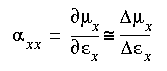
With this option, various properties can be studied in the presence of an electric field. In particular, the polarizability tensor can be computed by computing the dipole moment in the presence of electric fields in the x, y, and z directions.
Polarizabilities are in fact the first-order change of the dipole moment with respect to an external field, which may be estimated by computing the finite change to a dipole moment in the presence of a finite field:, e.g.
In practice, these polarizability terms require at least four separate calculations: one without a field and one with the field in each of directions x, y, and z. More reliable results are obtained if fields are applied in both the positive and negative directions and the results are averaged.
To impose an electric field of strength 0.001 atomic units in the y direction, enter:
Electric_Field 0.00 0.001 0.00
The Electrostatic_Moments keyword specifies to compute dipole moments.
Electrostatic_Moments value
Dipole moments are printed in both atomic units and Debyes.
The ESP_Charges keyword specifies to fit ESP charges.
ESP_Charges value
ESP charges can be frozen during optimization by providing explicit input in the espfit.inp file (see espfit.inp file).
Fixed fix coordinate specifications
The Fixed keyword is used to specify Cartesian constraints (i.e., to constrain the x and/or y and/or z coordinate(s) of specified atom(s)) that are to be enforced during a geometry optimization. The fix coordinate specifications are input on separate lines of the input file (immediately following the line containing the Fixed keyword) and are specified as:
atom x (and/or) y (and/or) z
Where the atoms are indexed by integers in the order in which they appear in the molecular geometry. The fix coordinate specifications must be terminated with a separate line containing only the string endfix immediately following the last fixed atom definition.
The Fixoc keyword specifies to fix (freeze) the orbital occupations for a specific number of cycles.
Fixoc value
DMol normally attempts to optimize the orbital occupations at each iteration. Fixoc stops it from optimizing the orbital occupations (i.e., freezes the orbitals) after n iterations. The default of 1000 insures that the program never freezes occupations.
An alternative way of freezing occupations is to enter the occupancy explicitly through a user-defined run_name.occup file.
The Frozen keyword is used for freezing core orbitals.
Frozen value
Core orbitals are atomic basis functions that are removed from the molecular orbital expansion and from the self-consistent procedure. They are thus analogous to effective potentials in Hartree-Fock calculations.
The default value results in a good compromise between cost and accuracy. Using the all_core keyword results in a significant reduction in computation time but may compromise the reliability of the results.
The use of effective potentials in Hartree-Fock theory is comparable to using these frozen core orbitals. Normally with such effective potentials, an entire shell is frozen. For example, the 2s and 2p would both be frozen on Na. In several test cases, freezing the 2p on silicon was found to create problems with geometry optimizations. For that reason, the Frozen inner_core option generally freezes fewer orbitals than would the corresponding effective potential Hartree-Fock calculation. The effects of using Frozen all_core on computational results have not been fully assessed.
More versatile combinations of frozen orbitals are possible by specifying the user option for the Basis keyword. See also the description of the fzminpol.dat file (Atomic information supplied with DMol) for a flexible way of introducing frozen orbitals. The open-shell 4f orbitals of the lanthanides and the 5f orbitals of the actinides should be left in valence space. This can be accomplished by changing the fzminpol.dat file or selecting the Basis user option.
The FrqRestart keyword restarts a frequency evaluation.
FrqRstart value
Evaluation of the Hessian by finite differences requires a separate calculation of the gradient for each atom perturbed in each direction x, y, and z. As each gradient is computed, it is stored in the .hess file.
If the calculation is interrupted, you can restart it, beginning with the next displacements, with the input:
FrqRestart on
thereby not wasting your previous results. DMol automatically searches the data in the .hess file, identifies the last atom and coordinate for which gradients are available, and restarts the calculation at the next finite displacement. If the .hess file contains all the gradients necessary to calculate the second derivatives, DMol uses the data in the .hess file to compute the vibrational frequencies and evaluate thermodynamic properties.
The Functionals keyword specifies the local correlation and gradient-corrected functionals for exchange and correlation.
Functionals value_keyword
Specifying one of these values for the Functionals keyword actually sets the appropriate values of the GC_Correlation, GC_Exchange, and Local_Correlation keywords. If the Functionals keyword is specified, these other keywords are ignored.
The local correlation functional vwn is the Vosko-Wilk-Nusair parametrization of Ceperley and Alder's electron gas Monte Carlo data.
The keyword basis allows you to run DMol calculations with whatever functional is specified in the basis set file. If no basis set file is present and the value of the Functionals keyword is basis, DMol performs a VWN calculation. The Insight, dialog, and dmol_master interfaces interpret basis as meaning the VWN potential and create a basis set file for the VWN potential. To predict the geometry of molecules with covalent bonds, the local vwn functional is recommended. To obtain reliable thermochemistry, specifying the bp functional, together with setting the Nonlocal keyword to energy, may be needed.
The value-keywords JMW, B88, and LYP are no longer valid for the Functionals command. However, the Hedin-Lundqvist/Janak-Morruzi-Williams local correlation functionals, Becke's 1988 version of a gradient-corrected exchange functional, and the Lee-Yang-Parr correlation functional can be specified by setting the values of the GC_Correlation, GC_Exchange, and Local_Correlation keywords separately.
The GC_Correlation keyword is used to select a gradient-corrected correlation functional.
GC_Correlation value_keyword
The pw functional is recommended, together with the b88 gradient-corrected exchange functional. This is equivalent to using Functionals bp.
The GC_Exchange keyword is used to select a gradient-corrected exchange functional.
GC_Correlation value_keyword
The b88 functional is recommended, together with gradient-corrected correlation pw functional. This is equivalent to using Functionals bp.
The GDIIS keyword specifies the maximum size of the subspace for the GDIIS procedure in geometry optimization.
GDIIS value
The GDIIS keyword is used to select the DIIS convergence procedure for geometry optimization, for example:
GDIIS auto
Note: GDIIS can be used only for optimizations to minima. Transition-state searches must be done with GDIIS off.
The Geometry keyword says where to read the molecular geometry and in what units.
Geometry where_keyword unit_keyword
[value_number ...
blank line]
The unit flag appears on the same line as Geometry, following the flag that tells DMol where to find the geometry. If the unit is left blank, then bohr is assumed.
If user is specified, the geometry is read starting on the next line. For each atom enter in free format:
X Y Z IZ
where X, Y, and Z are the Cartesian coordinates and IZ is the atomic number. Terminate this input with a blank line.
car is the only option available when the DMol input file is set up through the Insight interface.
The geometry for CH2 could be specified as:
Geometry		user	bohr
	0.0000000000	1.8900000000	1.89000000000	1
	0.0000000000	-1.8900000000	1.89000000000	1
	0.0000000000	0.0000000000	0.00000000000	6
<BLANK LINE>
The Gradient_Convergence keyword specifies the threshold for gradient convergence during geometry optimization.
Gradient_Convergence value
The geometry is considered converged to a minimum when the largest (in magnitude) component of the gradient vector is less than Gradient_Convergence. The geometry is considered optimized when the gradient convergence criterion is satisfied and either (or both) the displacement convergence or energy convergence criterion is satisfied (see Opt_Energy_Convergence, and Displacement_Convergence). The energy minimum does not correspond exactly to the point of zero gradient.
The Grid keyword specifies the grid on which the electronic properties specified by Plot are evaluated.
Grid value_keyword
[value_number ...]
The grid specified by Grid is different from the mesh used for numerical integration. Grid data are read only when Plot is used.
If the box option is used, the next line must contain the data (in free format):
ndim nx ny nz extnd
where:
- ndim = 3, the dimensionality of the plot (default = 3).
- nx, ny, nz = Grid spacing in the x,y,z directions (default = 5).
If > 0, these represent the actual grid size in units of 0.1 Å.
If < 0, these represent the number of spacings in each direction.
- extnd = The distance in angstroms that the grid extends beyond the molecule (default = 5.0 Å).
When the option user is chosen, you must specify an origin and two or three vectors that determine, in effect, the sides of the plane or box used for the grid. Unlike the box option, these vectors need not form a rectangular grid. The format is:
Grid	user
ndim	o1	o2	o3
nx	x1	y1	z1
ny	x2	y2	z2
nz	x3	y3	z3
where:
- ndim Dimensionality of the plot (3).
- o1, o2, o3 Origin of the grid in Cartesian coordinates (in Bohrs if you use .inmol file, angstroms if .input file).
- x1, y1, z1 Define a vector from the origin to the first corner
of the box.
- x2, y2, z2 Define a second vector from the origin.
- x3, y3, z3 Define a third vector.
- nx, ny, nz Number of grid spacings from the origin to each of the three points.
The three vectors defined in this way can be parallel to the x, y, and z Cartesian axes. However, this does not have to be so. This allows you to, for example, plot properties within a unit cell of a non-cubic system.
Important
Example 1
To construct a 3D plot with a grid spacing of 0.5 Å with the grid extending 10 Å beyond the molecule, enter the data:
	Grid	box
	3	5	5	5	10.0
Example 2
To construct a 3D plot with 20 X 20 X 20 grid points and the grid extending 5 Å beyond the molecule, enter the data:
	Grid box
	3	-20	-20	-20	5
This is a very dense grid, which produces very large files.
Example 3
To take a cross section through the carbon and one of the hydrogen atoms of CH2, but perpendicular to the plane of the molecule, you could use the input:
	Grid	user
	 2	-10.0	 0.0	 0.0
	30	 10.0	 0.0	 0.0
	30	-10.0	 1.89	 1.89
No equivalent input with the box option is possible in this case.
The Hessian_File keyword indicates the name of the file that contains the Hessian matrix.
Hessian_File value
The Hessian_File keyword is used for reading the starting Hessian matrix for the geometry optimization from a file, for example:
Hessian_File ../archive/ch3nh2.hessian
The file must contain a Hessian matrix in MSI .hessian file format (see File Formats documentation). The Hessian file can be generated using DMol or any other MSI quantum program that can run through the Insight interface. A DMol geometry always produces a new Hessian file that can be used to restart a run.
The Hessian_Update keyword controls how the Hessian matrix is updated during the calculation.
Hessian_Update value
The Hessian_Update keyword selects the method for updating the Hessian matrix during a geometry optimization, for example:
Hessian_Update BFGS
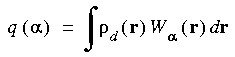
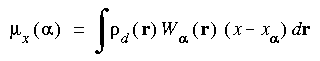
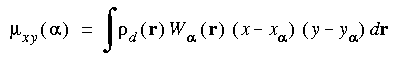
The Hirshfeld_Analysis keyword specifies atomic population analysis by the Hirshfeld partitioning procedure.
Hirshfeld_Analysis value ...
The Hirshfeld partitioned charges are defined relative to the deformation density. The deformation density is the difference between the molecular and the unrelaxed atomic charge densities and is given by:
where  (r) is the molecular charge density and a(r - R
 ) is the density of the free atom at coordinates R. Using the deformation density, the effective atomic charges, dipoles, and quadrupoles on atom are defined as (Delley 1986):
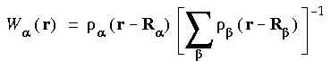
The weight W(r) is defined as the fraction of the atomic density from atom at coordinate r:
The Integration_Grid keyword controls the selection of mesh points for the numerical integration procedure used in the evaluation of the matrix elements. Since the functions in these equations are given numerically, the choice of mesh points can have a significant impact on the final results.
Integration_Grid value_keyword
[value_number ...
blank line]
A value of medium appears to give a reasonable compromise between computational expense and numerical precision. (Entering any value other than those listed above defaults to medium.)
A value of fine is used whenever difficulties are found with the medium mesh. Such problems can include discontinuous energies (i.e., bumpy rather than smooth potential energy surfaces are observed) and failure of a geometry optimization.
A value of xfine results in a nearly saturated mesh. This option is generally used only for benchmark calculations, not for day-to-day production runs.
A value of coarse results in lower computational cost and a significant reduction in the quality of the calculation. The results are at least qualitatively correct.
A value of xcoarse represents a serious compromise in the quantitative aspects of the calculation. It is useful for:
A value of user allows you complete flexibility in specifying the integration mesh. Six parameters are required to completely specify the integration mesh. The flags xcoarse, coarse, medium, fine, and xfine select predetermined values for them. The parameters are called ipa, iomax, iomin, thres, rmaxp, sp. The mesh is specified in spherical coordinates around each atomic center. The values of rmaxp and sp control the radial distribution of points, and iomax, iomin, and thres control the angular sampling.
Radial points are taken in shells from the nucleus out to a distance of rmaxp (default = 10.0 au). The number of shells is a function of the nuclear charge, so that heavier elements have a greater number of points. The actual number is 14 X (Z + 2)1/3, where Z is the atomic number. The value of sp may be used to increase or decrease this number, that is, sp = 2.0 results in twice as many radial points.
Angular sampling points are generated on each shell using a spherical harmonic function. The initial number of angular sampling points is 14, generated with a harmonic function with l = 5. The number of angular points must be increased at larger radii in order to maintain the quality of the numerical integration. The value of thres specifies the requested numerical precision (default = 0.0001), and the number of angular points is increased to maintain the precision. The minimum value of the harmonic generator is given by iomin (default = 1) and the maximum allowed value by iomax (default = 4). The value cannot increase beyond iomax, even if numerical precision is compromised.
The following table gives the angular momentum of the spherical harmonic function used to generate the points on a radial shell and the number of such points:
The value of ipa (default = 5) controls the partition function used to improve the convergence of the numerical integration. The ipa values correspond to Eqs. 24 (ipa = 0), 25 (1), 26 (2), 23 (5), and 27 (6).
The default values for each of these parameters that are selected by the flags xcoarse, coarse, medium, fine, and xfine:
To input values for these six parameters via the user option, begin immediately after the keyword Integration_Grid line and enter the data for npri, ipa, iomax, iomin, thres, rmaxp, and sp on a single line. (npri is an obsolete parameter and should always be 0.)
The following two inputs result in the same selection of mesh points for CH2:
Integration_Grid medium
or
Integration_Grid			user
0	5	5	1	0.0001	10.0	1.0
<BLANK LINE>
The Lmax keyword specifies multipolar fitting functions.
Lmax value ...
Lmax is used to specify the maximum angular momentum of the multipolar fitting functions that specify the analytical form of the charge density and the Coulombic potential. For each unique atom type (i.e., atomic number), enter the value of the desired maximum angular momentum for the fitting functions, in the same order as the atoms appear in the Geometry specification. Enter all values on the same line, following the keyword Lmax. Larger values of Lmax result in increased accuracy along with (a small) added computational cost. The default value of Lmax (which you obtain if you omit the Lmax line) is one greater than the maximum angular momentum in the atomic orbital basis. For most applications, the default Lmax values are satisfactory.
Consider Fe(C5H5)2. If the molecular geometry is specified in the order C C C C C H H H H H Fe, the Lmax specification for a minimal basis set is:
Lmax 2 1 3
which tells the program to use up to l = 2 (quadrupole-type) functions on C, only dipole functions on H, and up to l = 3 functions on Fe. The default specification in a DNP basis is:
Lmax 3 2 3
which tells the program to use up to l = 3 functions on C, quadrupole-type functions on H, and up to l = 3 functions on Fe.
Local_Correlation value
If the standard functional is used (Functionals keyword), the Local_Correlation keyword is ignored.
The Locate keyword specifies whether to perform transition-state search or minimization.
Locate value
The Locate keyword is used to select what type of stationary point to locate during the geometry optimization, for example:
Locate minimum
The actions of the options are:
- minimum:
- Geometry optimizer searches for a minimum on the molecular potential energy surface (i.e., a stationary point at which all eigenvalues of the Hessian matrix are > 0).
- transition_state:
- Geometry optimizer searches for a transition state on the molecular potential energy surface (i.e., a stationary point at which only one eigenvalue of the Hessian matrix is < 0).
The Lower_Energy_Limit keyword defines the lower bound of the transition energy range.
Lower_Energy_Limit value [units]
If Optical _Absorption is on, the Lower_Energy_Limit and Upper_Energy_Limit keywords control the range of energies within which electronic transitions are computed.
The Rydberg is a fundamental spectroscopic unit (the energy difference between the hydrogen atom 1s ground state level and the continuum is one Rydberg, or half a Hartree).
However, DMol in the Insight interface writes units to the input file as cm-1. The actual values used in the calculation are reported at the top of the run_name.outmol file.
The Max_Displacement keyword specifies the maximum allowed step size.
Max_Displacement value
The Max_Displacement keyword is used to specify the maximum length of the geometry update vector, for example:
Max_Displacement 0.2
The value set is the maximum allowed length of the geometry update vector; if the displacement would be larger than real, the step is scaled. For transition-state searches, smaller displacements are recommended (<0.003), especially when no Hessian information is present but the geometry is close to the transition-state geometry.
The Mixing_Alpha keyword specifies the mixing coefficient for the charge density.
Mixing_Alpha value
The mixing coefficient restricts the maximum allowed change in the charge density each iteration of the DFT self-consistent procedure. If old is the charge density from the previous iteration and curr is the density in the current iteration, then the new density is:
This results in smoother convergence.
During this procedure, DMol actually uses several previous densities and performs an interpolation or extrapolation. If the interpolation is found to be too nonlinear, the value of Mixing_Alpha may be temporarily reduced during an iteration. Specifying a negative value of Mixing_Alpha eliminates this temporary reduction and forces simple mixing to occur as in the above equation (but using the absolute value of Mixing_Alpha).
For systems with a large number of low-lying excited states such as metal clusters, it is not unusual to have values of Mixing_Alpha as small as 0.005.
When oscillatory behavior is observed rather than convergence during the DFT self-consistent procedure, the value of Mixing_Alpha should be decreased.
The Mixing_Beta keyword specifies the mixing coefficient for the spin density.
Mixing_Beta value
The mixing coefficient restricts the maximum allowed change in the spin density each iteration of the DFT self-consistent procedure. If old is the spin density from the previous iteration and curr is the density in the current iteration, then the new density is:
This results in smoother convergence.
During this procedure, the program actually uses several previous densities and performs an interpolation or extrapolation. If the interpolation is found to be too nonlinear, the value of Mixing_Beta may be temporarily reduced during an iteration. Specifying a negative value of Mixing_Beta eliminates this temporary reduction and forces simple mixing to occur as in the above equation (but using the absolute value of Mixing_Beta).
For systems with many low-lying excited states, such as metal clusters, you may need values of Mixing_Beta as low as 0.005.
When oscillatory behavior is observed rather than convergence during the DFT self-consistent procedure, the value of Mixing_Beta should be decreased.
The Mulliken_Analysis keyword specifies atomic population analysis by the Mulliken method.
Mulliken_Analysis value ...
For a simple Mulliken (1955) analysis (Mulliken_Analysis 1), the total effective number of electrons in each atomic orbital is printed. Following this is a reduced or condensed population analysis, giving the total number of electrons in each type of orbital. For example, when using a DN basis, the population analysis gives occupations for two 2s functions, and two 2p functions (for each ml) on every atom. The reduced analysis gives just one 2s, and one 2p population. Following these values comes the effective charge for each atom.
When a population overlap matrix is specified (Mulliken_Analysis 2), the orbitals span only the reduced or condensed orbitals; that is, there is only one entry for 1s, 2s, 2p, etc. on each atom, regardless of the size of the atomic basis set.
Requesting both Mulliken analysis and a population overlap matrix (Mulliken_Analysis 3) results in the effective number of electrons associated with each pair of atomic orbitals.
Frozen core orbitals necessarily have an occupation of 2. They are not included in the population analysis.
The NDiff keyword specifies number of finite differences of gradients used in frequency evaluation.
NDiff value
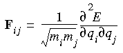
Harmonic vibrational frequencies are computed by diagonalizing the mass-weighted second-derivative matrix, F (Wilson et al. 1980). The elements of F are given by:
Here, qi and qj represent two Cartesian coordinates of atoms i and j, and mi and mj are the masses of the atoms. The square roots of the eigenvalues of F are the harmonic frequencies.
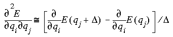
In DMol, it is not possible to compute the second derivatives analytically, so they are computed by finite differences of first derivatives. Gradients are computed at displaced geometries and second derivatives are computed numerically.
A value of 1 for NDiff uses single-point differencing for this process. Displacements are taken in only one direction:
where the two terms represent the analytic derivatives at the equilibrium geometry and at a geometry with coordinate qj displaced by distance  .
.
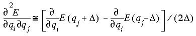
A value of 2 for NDiff uses two-point (or central) differencing to obtain the second derivatives:
This can reduce numerical rounding-off errors, but takes twice as much computer resources as single-point differencing.
The Nonlocal keyword indicates how to include nonlocal functionals.
Nonlocal value_keyword
A value of energy causes the gradient-corrected "nonlocal" exchange and correlation energies to be calculated as a perturbation on a converged LDA density. This is a single calculation done at the end of an LDA calculation. A value of potential causes the gradient-corrected functional to be applied self-consistently. The potential option is usually more time-consuming than the energy option. If no nonlocal functional is selected, the Nonlocal keyword is ignored.
The Nuclear_EFG keyword specifies calculation of the electric field gradients at nuclei.
Nuclear_EFG value
When Nuclear_EFG is on, electric field gradients are calculated at the positions of all symmetry-unique nuclei.
The Number_Bad_Steps keyword specifies the number of allowed bad (divergent) iterations before aborting a run.
Number_Bad_Steps value
During the self-consistent procedure, if the mixing factor is too large, the iterations might not converge. Number_Bad_Steps indicates how many bad steps in a row are permitted before the program aborts the self-consistent procedure. Values of 0 or 1 are not recommended, since the program often takes a single divergent step but recovers on the next iteration.
This option allows you to specify a very large number of iterations (large values of SCF_Iterations) without risking that DMol might simply oscillate for a great many iterations, wasting CPU time without converging. This option insures that the run aborts rather than continuing to waste time.
The Occupation keyword specifies orbital occupations.
Occupation value_keyword
[value_number ...]
If valence or total is specified, the occupations are entered, starting on the next line, as:
N oc od
where N (an integer) indicates the number of orbitals having this occupation, oc (real number) is the spin-up (alpha) orbital occupation number, and od (real number) is the spin-down (beta) orbital occupation. Terminate the occupation for each irreducible representation with a line containing only a 0. (If you are not using symmetry, there is only one irreducible representation.)
The triplet state of the CH2 molecule has three doubly occupied and two singly occupied orbitals. If you are not using symmetry, specify the input as:
Occupation		TOTAL
3	1.0	1.0
2	1.0	0.0
0
If you are using C2v symmetry, then the occupation of CH2 is 1a12 2a12 3a11 1b11 1b22. The a2 block is unoccupied. The occupation can be specified as:
Occupation total
2	1.0	1.0
1	1.0	0.0
0
0
1	1.0	0.0
0
1	1.0	1.0
0
The order of the representations (a1 a2 b1 b2) is the same as in Cotton (1971) and a list is always printed in the outmol file. Occupations for unused representations should not be specified, and for degenerate representations one should specify occupations only for the first representation.
The program writes an .occup file during the SCF cycles. The fromat of the file is as explained above.
The Opt_Coordinate_System keyword specifies the kind of coordinate system.
Opt_Coordinate_System value
The Opt_Coordinate_System keyword is used to select the coordinate system in which to carry out the geometry optimization, for example:
Opt_Coordinate_System internal
The Opt_Cycles keyword specifies the number of geometry optimization cycles.
Opt_Cycles value
Geometry optimizations are performed by evaluating a gradient, followed by a Hessian update and calculation of a new set of coordinates. The value of Opt_Cycles controls the number of complete iterations that are performed in a DMol run. Opt_Cycles is used only if an optimization is requested, i.e., if the optimize_frequency or optimize option is specified for the Calculate keyword.
The Opt_Energy_Convergence keyword specifies the threshold for energy convergence during geometry optimization.
Opt_Energy_Convergence value
The Opt_Energy_Convergence keyword is used to specify the geometry optimization convergence criterion for the total molecular energy. The energy criterion is met if the difference between the total energy in two consecutive optimization steps is less than real. The geometry is considered optimized when the gradient convergence criterion (Gradient_Convergence keyword) is satisfied and either (or both) of the displacement convergence criterion (Displacement_Convergence) or energy convergence criterion is satisfied. Recall that the energy minimum does not correspond exactly to the point of zero gradient.
The Opt_Print keyword controls the printout.
Opt_Print value
The Opt_Use_Symmetry specifies whether to use symmetry during the calculation.
Opt_Use_Symmetry value
The Opt_Use_Symmetry keyword is used to select whether molecular symmetry will be used in the context of the geometry optimization, for example:
Opt_Use_Symmetry on
When on is specified, all quantities used by the optimizer (Hessian matrix, geometry update vector, etc.) will be restricted to the symmetry of the molecule. Thus, the molecule will maintain its initial symmetry throughout the optimization.
Using symmetry in the optimization is independent of using symmetry in the SCF calculation (Symmetry keyword).
The Optical_Absorption keyword controls the calculation of optical absorption spectra in DMol.
Optical_Absorption value
If Optical_Absorption is on, the Lower_Energy_Limit and Upper_Energy_Limit keywords control the range of energies within which electronic transitions are computed.
Setting the Partial_DOS keyword causes the partial density of states coefficients to be written to a run_name.dos file.
Partial_DOS value
The partial density of states can be displayed by using the Analysis/Density_of_States command in the Insight interface.
The Plot keyword specifies how to compute electronic properties for plotting.
Plot value_keyword [# ...] ...
Plot causes DMol to generate values of various electronic properties on a 2D or 3D grid for subsequent plotting.
To generate the values for plotting any of the above options, enter Plot followed by the value keyword. More than one value keyword can be included on one line; however, if the orbital value is used, orbitals must be specified as the last values in the line or on a separate line. To plot orbitals, enter the orbital number(s) after the word orbital.
Orbitals are numbered from lowest to highest orbital energy. Core orbitals are not included in the numbering and can not be plotted.
To plot the total density, the electrostatic potential, and orbitals 7, 8, and 9, enter:
Plot density potential
Plot orbital 7 8 9
The Point_Charges keyword specifies to include point-charges in the calculation.
Point_Charges value
Point charges can be used to simulate the chemical environment due to a large molecule or crystal. The validity of such a calculation depends, of course, on the validity of the point-charge model and the choice of charges used.
Point charges are read in from a .car file.
Point charges can be used in combination with point group symmetry. You need to make sure, however, that the symmetry used in the calculation is a subgroup of the symmetry of both the central molecule and the point charge system.
Synonym of Mulliken_Analysis keyword. Population_Analysis on is equivalent to Mulliken_Analysis 1. Population_Analysis off means not to do Mulliken population analysis.
The Print keyword controls what data are printed to the .outmol file.
Print value_keyword ...
Each option may be abbreviated to its first three letters. More than one value can be specified on a line.
To print everything possible, use the input:
Print psi eig
The Project keyword specifies to project out translations and rotations from the force-constant matrix.
Project value
Normally, when vibrational frequencies are evaluated, there are 6 modes that have a value of zero, corresponding to the 3 translational and 3 rotational degrees of freedom. When a force-constant (second-derivative) matrix is not evaluated at the point of zero gradient, this is not necessarily true. However, it is possible to project the space of the translations and rotations from the force-constant matrix, forcing 6 zero eigenvalues. This has a slight effect on the remaining 3N - 6 vibrational frequencies.
The SCF_Density_Convergence keyword specifies the density convergence threshold for SCF.
SCF_Density_Convergence value
The SCF_Density_Convergence keyword is used to specify the electron density convergence threshold for the SCF procedure, for example:
SCF_Density_Convergence 0.000001
The SCF electron density is considered converged when the difference between the norm of the density matrices from two successive SCF iterations is less than the value of SCF_Density_Convergence. Either the energy (see SCF_Energy_Convergence keyword) or density convergence criterion must be satisfied for SCF convergence to be achieved.
The SCF_Energy_Convergence keyword specifies the energy convergence threshold for SCF.
SCF_Energy_Convergence value
The SCF procedure is halted when the degree of convergence is less than the convergence threshold or when the number of iterations is exceeded, whichever comes first. The degree of convergence is measured by the change in the total energy from one iteration to the next. Energy convergence is less commonly used than density convergence; therefore, SCF_Energy_Convergence = off by default.
The SCF_Iterations keyword is the maximum number of iterations.
SCF_Iterations value
Setting SCF_Iterations to larger values results in fuller convergence but added expense. The program exits when the number of iterations is exceeded or when the convergence criterion specified by SCF_Energy_Convergence or SCF_Density_Convergence is met, whichever comes first.
The SCF_Restart keyword is used to restart an interrupted or unconverged calculation.
SCF_Restart value
Because the .tpotl file contains the analytic representation of the Coulombic potential, restarting from it allows the SCF iterations to pick up where they left off. Alternatively, using an old .tpotl file at a different geometry may give the calculation a better starting guess than the default, the density from the superposition of atomic densities. If the integration grid, symmetry, or basis set is changed, the .tpotl file will no longer be compatible.
The Smear keyword specifies to perform charge smearing at the Fermi level.
Smear value
The Smear parameter allows electrons to be smeared out among all orbitals within a given E of the Fermi level. This procedure improves convergence of the SCF procedure by allowing orbitals to relax more rapidly. The character of the virtual orbitals can be more effectively mixed into the occupied space, since these orbitals are now fractionally occupied.
Specifying Smear real as input (real is a floating-point number) causes charge smearing among all orbitals within real Hartrees of the Fermi level. Typically, real ranges from approximately 0.001 to 0.1. In addition, the value of Smear should be less than the value of Mixing_Alpha or Mixing_Beta by a factor of about 2-10.
The Solvate keyword specifies the computation of solvent effects.
Solvate value
Specifies whether or not to perform a COSMO (COSMO--solvation effects) calculation.
The Spin keyword controls spin-restricted/unrestricted wavefunctions.
Spin value
For spin-restricted wavefunctions, the same orbitals are used for the alpha and beta electrons. For spin-unrestricted wavefunctions, different orbitals are used for different spins.
Closed-shell systems are run with spin-restricted wavefunctions and open-shell systems with unrestricted wavefunctions.
The symmetry keyword is used to input the point group symmetry for the molecule. Note: DMol cannot use the Symmetry keyword in conjunction with frequency or optimize_frequency calculations.
Symmetry value_keyword
The coordinates for the molecule need to be oriented according to certain conventions. This can be done from the Insight interface using the Find_Pt_Group command or using the standalone snap_to_sym utility. When the AUTO keyword, DMol detects the symmetry and transforms the coordinates automatically.
A file with the suffix .symdec is created. The .symdec file contains information on how to assemble symmetry orbitals (SO) from the atomic basis set. For a detailed explanation of molecular symmetry as implemented here, see Cotton (1971).
The use of symmetry offers several computational advantages. First of all, the secular equation becomes block diagonal. This reduces the size of the matrix diagonalization and subsequently speeds up the calculation. In addition, orbital occupation may be specified for each irreducible representation--this allows the investigation of electronic states of different symmetry. Finally, fewer numerical integration points need to be generated by the program. The points are generated only for a unique region of space, and the full set of points is obtained by symmetry operations. This reduces the computation time and disk storage requirements.
At present, the following limitations are imposed on the use of symmetry:
The TS_Mode keyword specifies the Hessian mode being followed during a transition-state search.
TS_Mode value
The Upper_Energy_Limit keyword defines the lower bound of the transition energy range.
Upper_Energy_Limit value [units]
If Optical _Absorption is on, the Lower_Energy_Limit and Upper_Energy_Limit keywords control the range of energies within which electronic transitions are computed.
The Rydberg is a fundamental spectroscopic unit (the energy difference between the hydrogen atom 1s ground state level and the continuum is one Rydberg, or half a Hartree).
However, DMol in the Insight interface writes units to the input file as cm-1. The actual values used in the calculation are reported at the top of the run_name.outmol file.
The Vibdiff keyword specifies the step size for finite differences.
Vibdiff value
For very flat potential energy surfaces, larger values of Vibdiff may be needed. Smaller values may be appropriate for steep surfaces.
Last updated September 25, 1997 at 03:16PM PDT.
Copyright © 1997, Molecular Simulations, Inc. All rights
reserved.

 0
0

 0
0